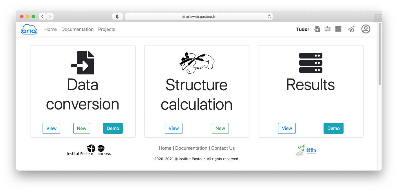
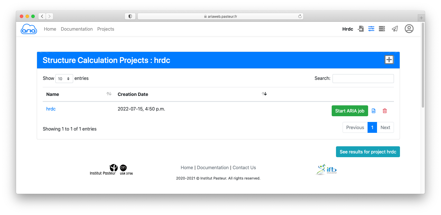
Once you have access to ARIAweb, here is how your homepage looks like.

In this practical, we will calculate the structure of a HRDC domain (Liu et al., 1999, Structure 15;7(12):1557-66) with ARIA2. The data comprise two NOESY spectra, torsion angles from 3J coupling constants and hydrogen bond restraints.
Links:
Once you have access to ARIAweb, here is how your homepage looks like.

In this tutorial, we will see how to use a starting model (e.g. from a previous calculation or from AlphaFold prediction) to help assigning NOEs. In turn the starting model(s) will mimic a previous iteration before iteration 0. Distances for possible NOE assignment will be measured used the coordinates the starting model(s) and used for calibration, elimination of spurious cross-peaks and unlikely assignment possibilities.
6. Advantage of using an input model
To predict a 3D model of our protein of interest, we will use this ColabFold notebook.
In the query_sequence filed, input the one-letter sequence of the construct used for NMR experiment, i.e. including the expression tag:
MKHHHHHHPMELNNLRMTYERLRELSLNLGNRMVPPVGNFMPDSILKKMAAILPMNDSAFATLGTVEDKYRRRFKYFKATIADLSKKRSSE
In the jobname field, enter hrdc and set num_relax to 1. Since we will use this model to evaluate inter-proton distances from NOE cross-peaks assignments, it is necessary to have a protonated model at the end and that is exactly what the relaxation with amber does.

Next, in the top menu of the ColabFold notebook, click Runtime > Run all. In the popup window, click Run anyway.
If you scroll down to the > Run Prediction section, you will see the predicted models as they are generated by AlphaFold.
After a few minutes, when all 5 models are generated, the notebook will generate a ZIP file (xxx.results.zip) to be saved. It will contains the predicted models along with some statistics. After unzipping the ZIP file, you will get the following files:
hrdc_5687f/
  |__cite.bibtex
  |__config.json
  |__hrdc_5687f.a3m
  |__hrdc_5687f.csv
  |__hrdc_5687f.done.txt
  |__hrdc_5687f_coverage.png
  |__hrdc_5687f_env
  |__hrdc_5687f_pae.png
  |__hrdc_5687f_plddt.png
  |__hrdc_5687f_predicted_aligned_error_v1.json
  |__hrdc_5687f_relaxed_rank_001_alphafold2_ptm_model_3_seed_000.pdb
  |__hrdc_5687f_scores_rank_001_alphafold2_ptm_model_3_seed_000.json
  |__hrdc_5687f_scores_rank_002_alphafold2_ptm_model_5_seed_000.json
  |__hrdc_5687f_scores_rank_003_alphafold2_ptm_model_4_seed_000.json
  |__hrdc_5687f_scores_rank_004_alphafold2_ptm_model_2_seed_000.json
  |__hrdc_5687f_scores_rank_005_alphafold2_ptm_model_1_seed_000.json
  |__hrdc_5687f_unrelaxed_rank_001_alphafold2_ptm_model_3_seed_000.pdb
  |__hrdc_5687f_unrelaxed_rank_002_alphafold2_ptm_model_5_seed_000.pdb
  |__hrdc_5687f_unrelaxed_rank_003_alphafold2_ptm_model_4_seed_000.pdb
  |__hrdc_5687f_unrelaxed_rank_004_alphafold2_ptm_model_2_seed_000.pdb
  |__hrdc_5687f_unrelaxed_rank_005_alphafold2_ptm_model_1_seed_000.pdb
  |__log.txt
The output files are:
log.txt: log file that contains the scores (ptm, plddt etc)*.pdb: PDB predictions for the 5 models, ranked by plDDT*.json: statistics of each model in json formathrdc_5687f_coverage.png: coverage of MSAhrdc_5687f_plddt.png: plDDT score along the sequencehrdc_5687f_pae.png: PAE plot for the 5 modelshrdc_5687f.a3m: MSA generate with MMseqs2 used for predictionThe model we will use for the rest of the tutorial is hrdc_5687f_relaxed_rank_001_alphafold2_ptm_model_3_seed_000.pdb. It is the best ranked model and the one that has been relaxed and protonated with Amber.

Before all, you will need to create a new project. First, go the ARIAweb homepage https://ariaweb.pasteur.fr/ and log in.
To run ARIA, you will need:
ARIA can import NMR data from various NMR formats (requires a conversion step) or directly from a CCPN project. The first option is the one described in this part of the tutorial, by first converting the data from various format to the internal ARIA XML format.
Since the original data are not stored in ARIA XML format, the first thing that needs to be done is to convert the NOE spectrum files from the original XEASY format to the ARIA XML format. The conversion routines check the data for consistency, and convert the atom names to strict IUPAC convention. ARIA uses the XML format to describe and store most of the crucial input files.
For this tutorial, we will load the corresponding data simply by clicking on the button.
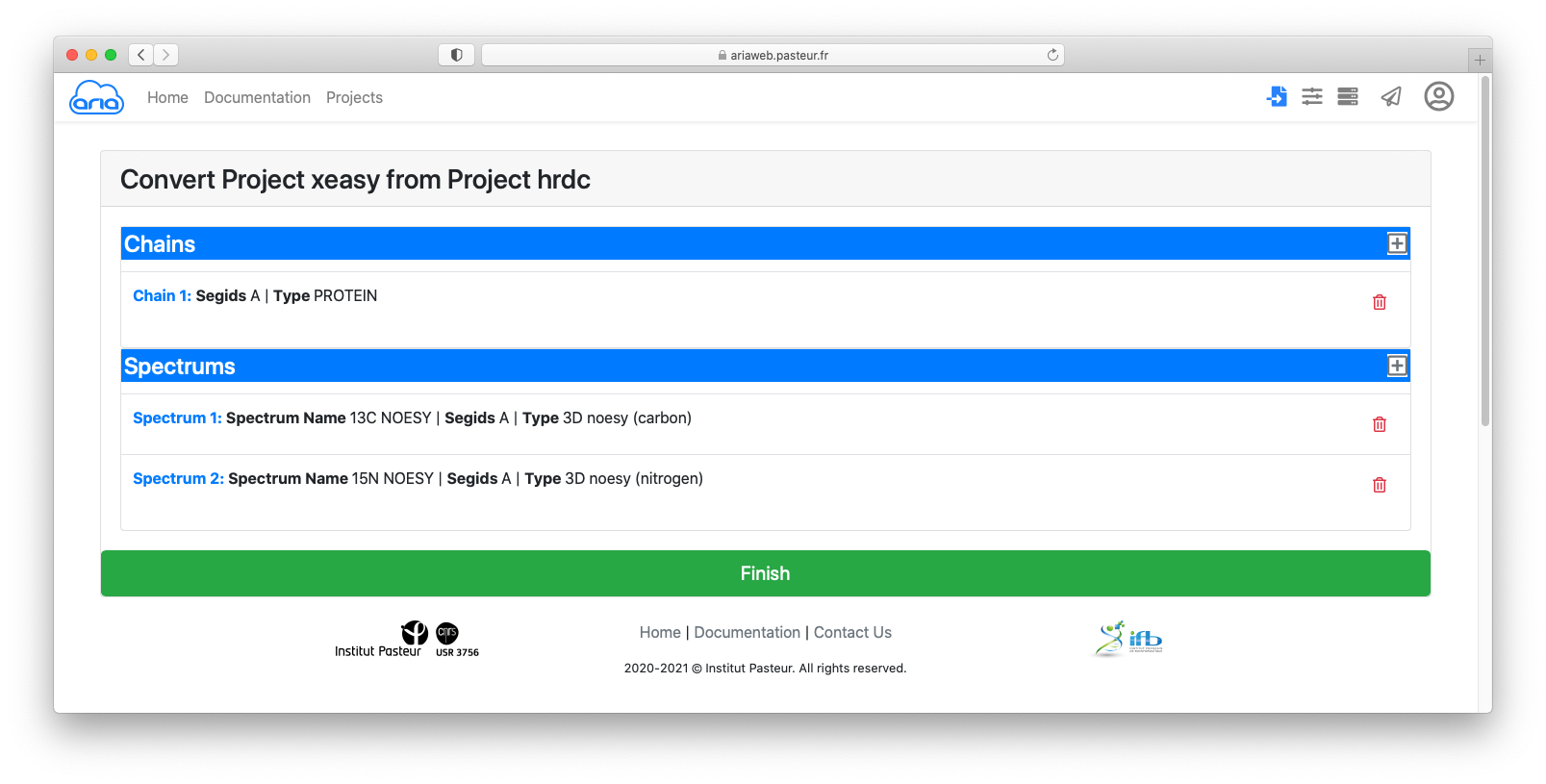
You can see that the data contain:
By clicking on each item (in blue), you can see details that must specified for conversion from Xeasy format to ARIA XML format.
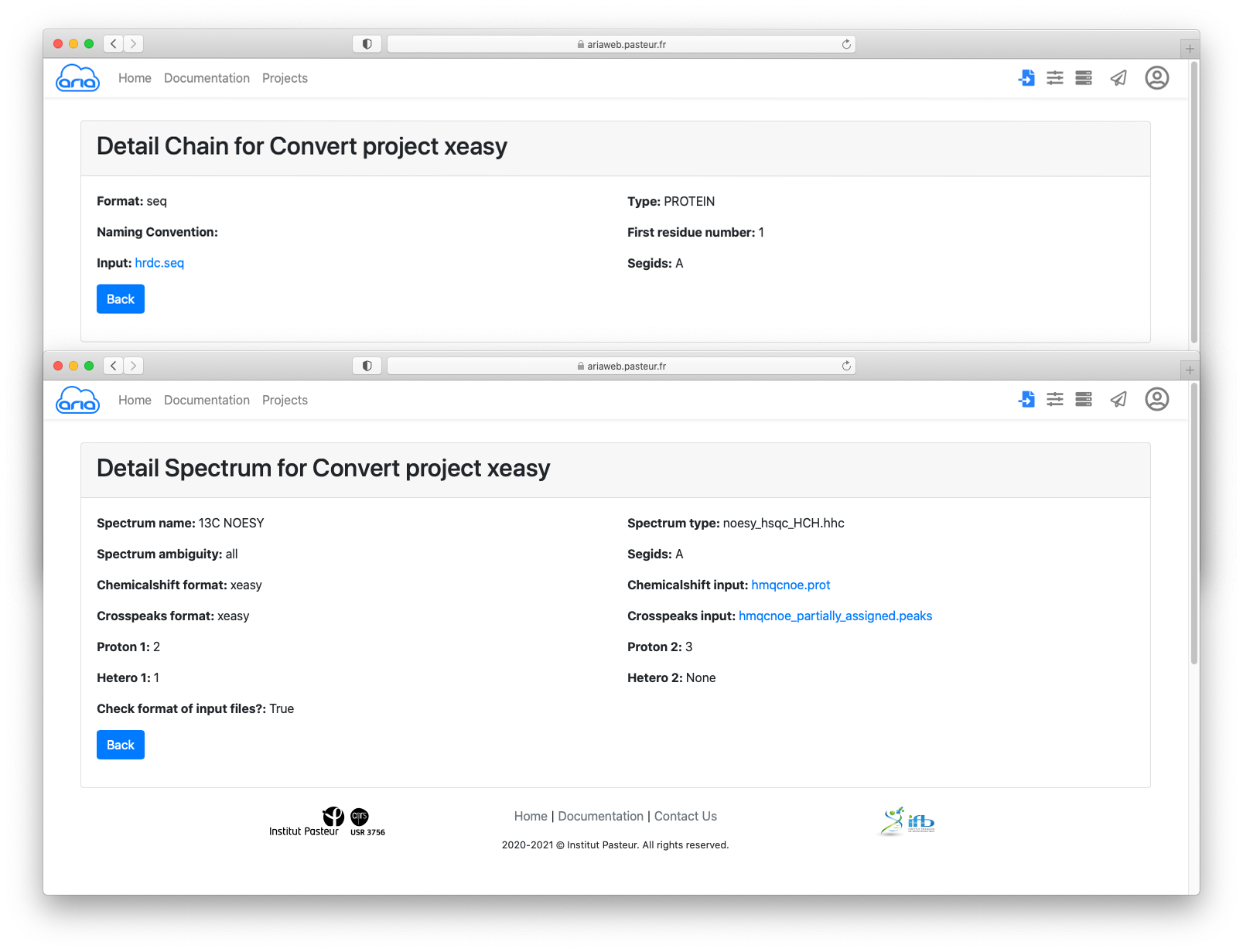
You can also have a look at the input files by clicking on the filenames (in blue) for the sequence, chemical shifts and cross-peak lists.
After clicking the button, you can save the conversion project by clicking on (Figure 5).
You will be then redirected to the page where you can submit the conversion data conversion on the server.

Click the button to submit you data conversion. You will be redirected to a Results page where you can see the status of your conversion job. See here for an explanation on the status icon (Figure 8).

The status icon indicates that he conversion job is running. Once the job is finished (status icon ), and if needed, you can download the convert files using the icon (Figure 9).
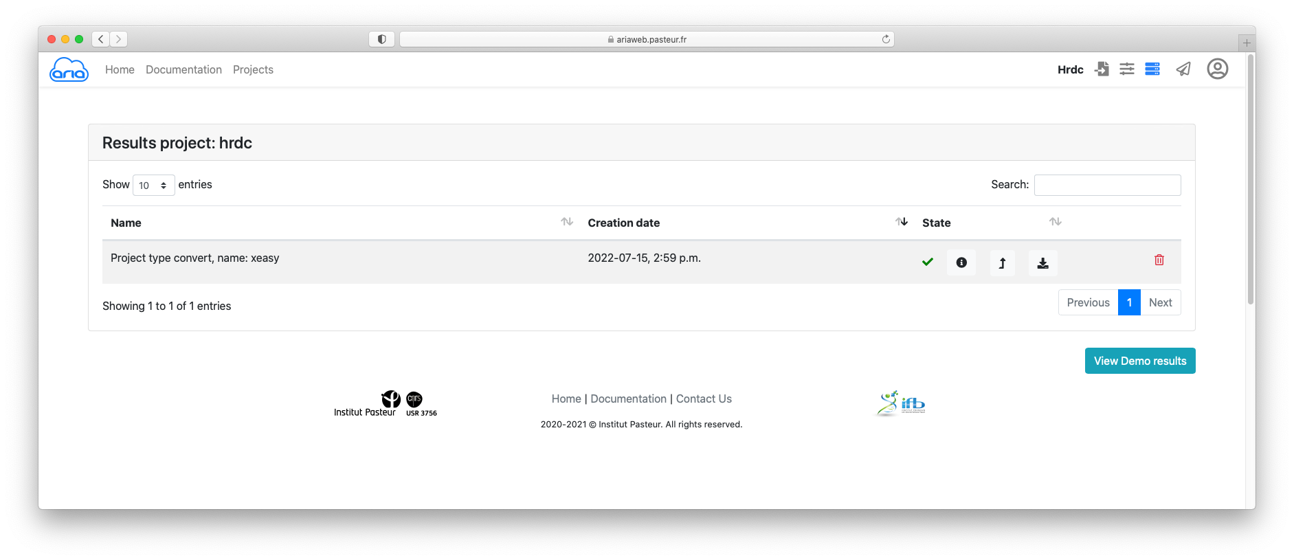
Now that you have converted your sequence and NOE data, you can prepare your ARIA structure calculation. ARIAweb allows to directly create a structure calculation project using the convert data by simply clicking on the button (Figure 9).
You now have a new form where you will be able to validate or modify all the parameters for your ARIA run. The Structure Calculation form is designed to guide the user through the main categories of parameters that need to be checked (if default values are used) or specified (if a user wants to change with customized values). The 4 main categories of parameters are:

Start by giving a name to this ARIA job, e.g. hrdc.
Click the button to move to the next section of the form.
In the DATA section, you will see that the molecular system is already pre-filled with your converted file form the previous step. Click to move to the Spectra definitions.
Again, your 13C-NOESY and 15N-NOESY peak-lists are already specified as 2 spectrum items with the files you converted before.
For the 2 spectra (scroll down to access Spectrum 2), uncheck the Use assignments box. Here we will not use any previous assignments (from manual analysis of the peaks).
Leave all parameters as default.
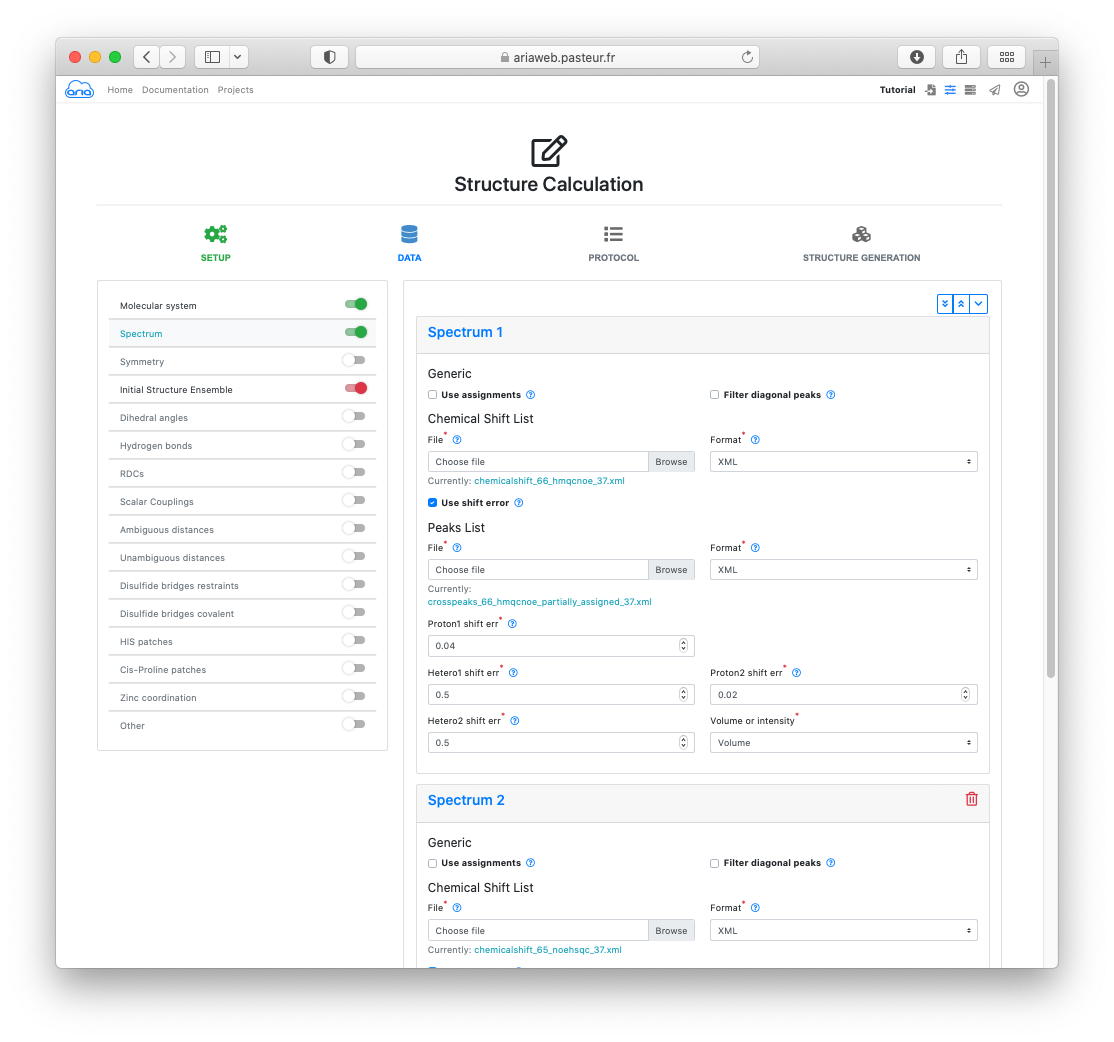
We will use the AlphaFold model to help the initial NOE assignment. To do so, activate the slider on the left for Initial Structure Ensemble (Figure 12).
Click the button to move to Initial Structure Ensemble.
Now click the button and select the AlphaFold model (hrdc_5687f_relaxed_rank_001_alphafold2_ptm_model_3_seed_000.pdb) so that it can be uploaded. Make sure to select the relaxed PDB file.
Select IUPAC for the Format.

Click the button to move to the PROTOCOL section.
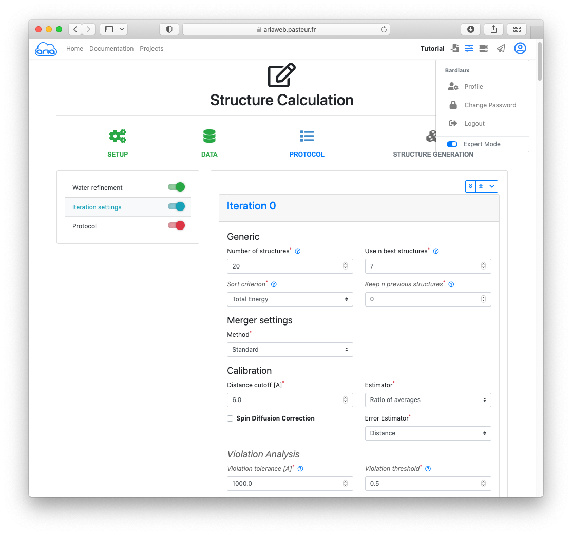
Since we will be using an initial input model, we need to adapt some parameters related to the stringency of the automated assignment method. To do so, you must enable the Expert mode from your User menu ( icon, top right).
Activate the slider on the left for Iteration settings (Figure 13).
On the Water refinement page, click the button to move to the Iteration settings.
For the first 3 iterations, we will change the following parameters:
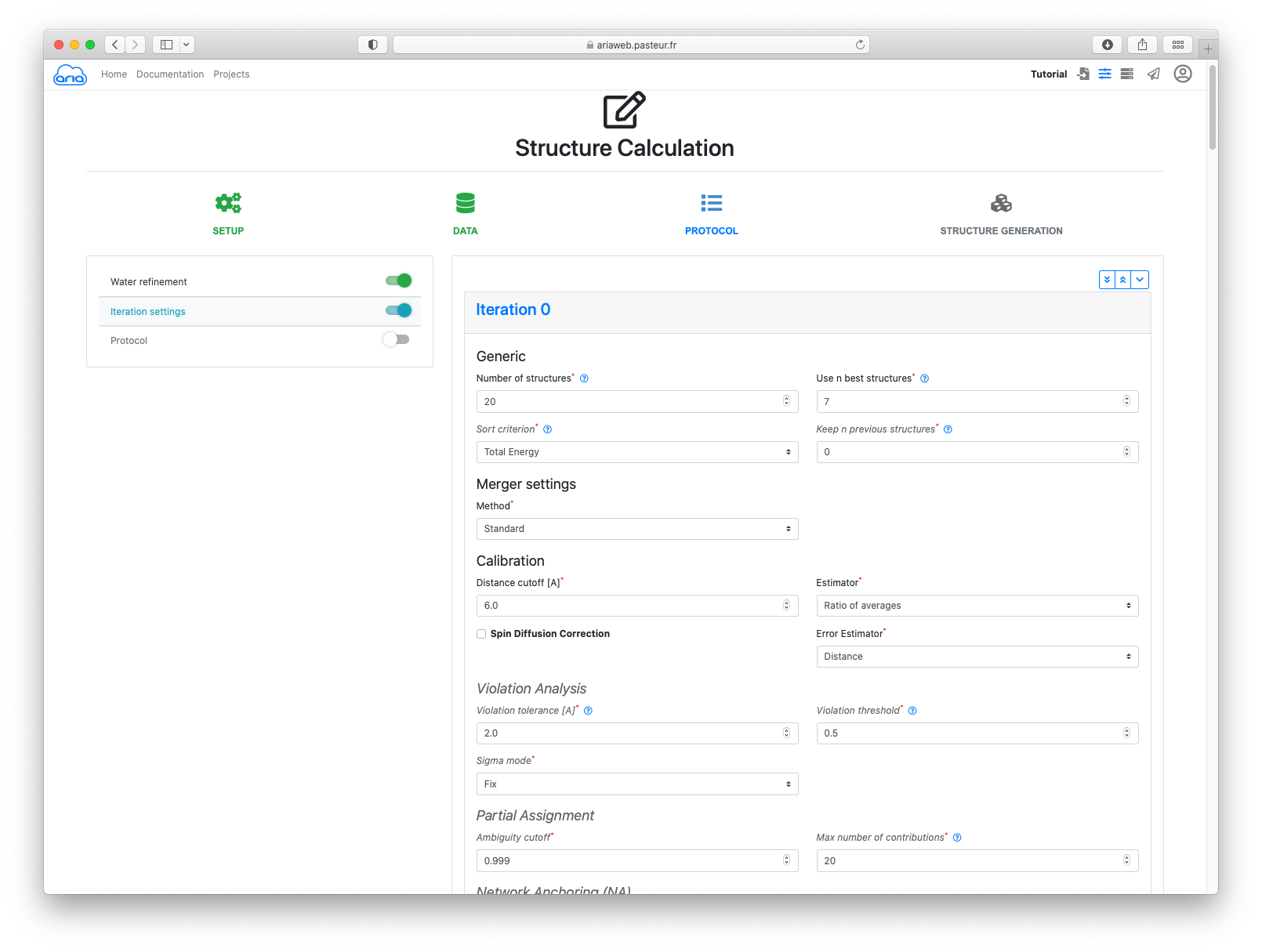
Set the following values for Iteration 0, 1 and 2 (scroll down to access other Iterations):
| Iteration | Violation tolerance | Ambiguity cutoff |
|---|---|---|
| 0 | 2.0 | 0.999 |
| 1 | 1.0 | 0.99 |
| 2 | 1.0 | 0.99 |
Scroll down to the bottom of the page and click the button again.
For the practical, we use all parameters as default for STRUCTURE GENERATION. Continue clicking until you see the button.
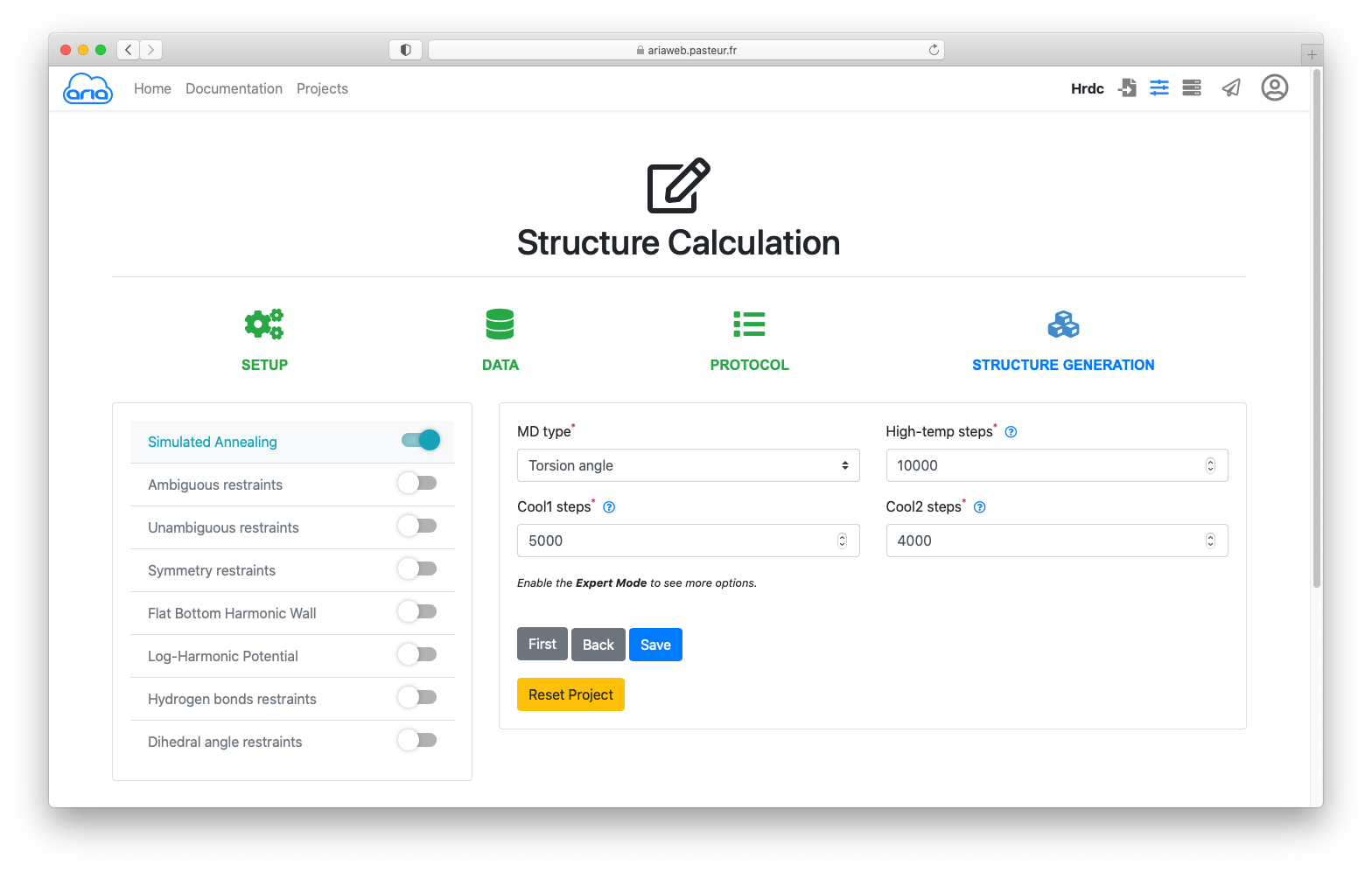
Clicking will save (no surprise here) your parameters and you will be directed to the page where can submit the ARIA calculation job.
Click the button to submit you structure calculation. You will be redirected to a Results page where you can see the status of your ARIA job. See here for an explanation on the status icon.
Depending on the server load the calculation might take ~30 minutes to hours... For the rest of the practical you will not have to wait until the calculation is finished. We have pre-calculated results that will allow you to visualise and analyse the results of an ARIA job.
When your job is finished (status icon ), click on the button to start the job analysis and visualize the results.
Results archive can be downloaded using .
The visualisation page allows to view an analysed the results of a structure calculation job. Final structure ensemble generated by ARIAweb are displayed interactively, with various representations. Final restraints statistics, structure quality checks and bundle RMSD are shown to help the user interprets the reliability of the results. On top of that, more graphs, restraints validation and PDB files can be downloaded directly (Figure 17).
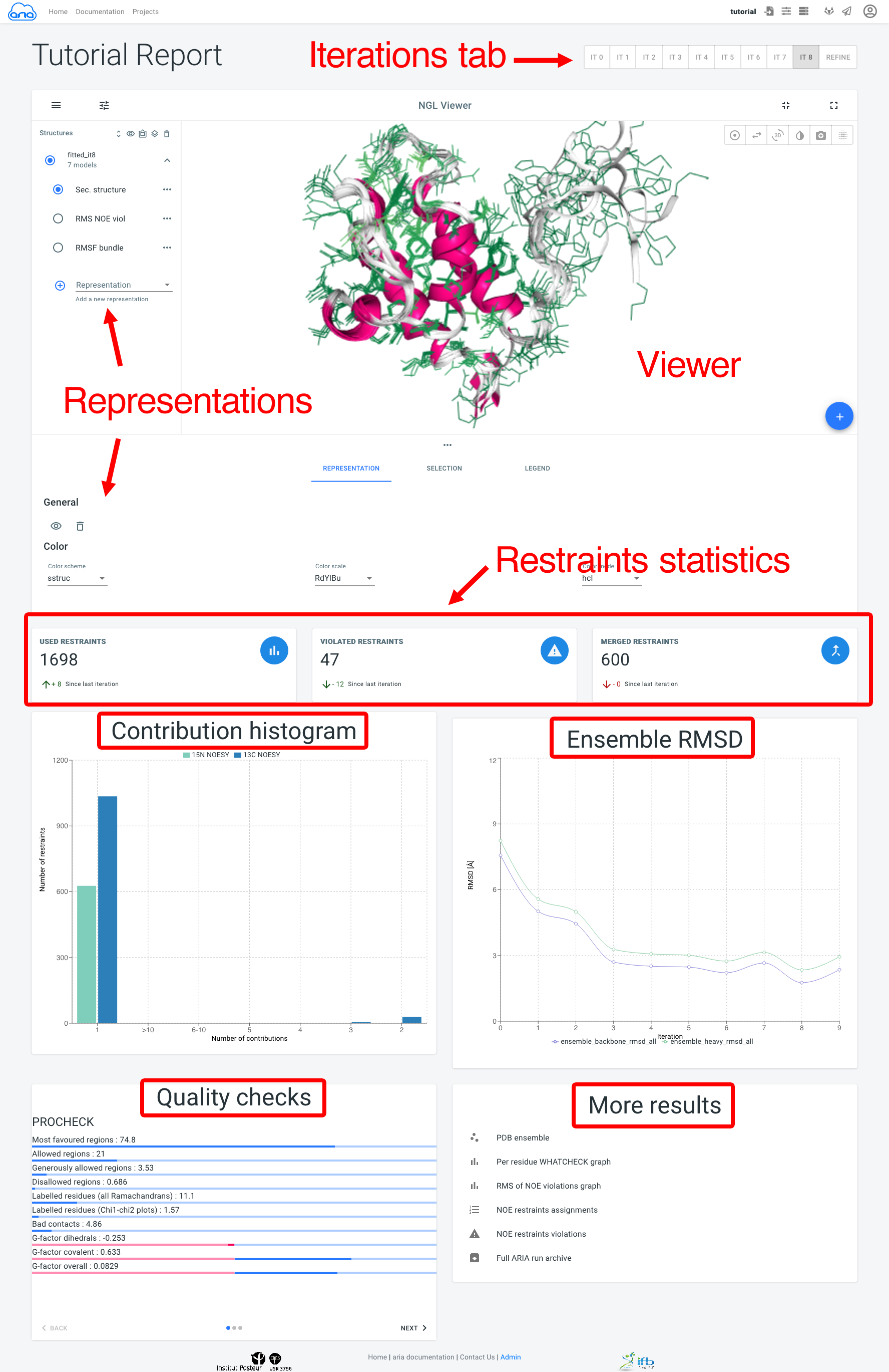
Results for all ARIA iterations can be shown by selecting an iteration in the Iterations tab. The main component of the Visualisation page is the NGL viewer. By default, several representations of the structure ensemble generated by ARIA are shown:
The Representation tab (below the NGL viewer) allows to change the visibility, styling and coloring of a selected representation. By default, all structures in the bundle are shown; use the filter_frames button to select individual models for display).
The add_circle button allows to upload another PDB file to superimpose on the ARIA structure ensemble (use the layers button to superimpose on a selected structure).
Below, Restraints statistics recapitulate the number of restraints and the trend since the previous iteration for:
The Contribution histogram gives count of restraints (from each input spectra) that have 1 (i.e. unambiguous) or more (i.e. ambiguous) assignment possibilities (or "contributions"). Ultimately, ARIA tries to reduce the ambiguity in NOE assignments, producing more unambiguous restraints. Truly ambiguous assignments can remain due to spectral overlap or chemical shifts degeneracy.
The Ensemble RMSD graph shows, for each iteration, the RMSD of the structure ensemble generated by ARIA ("bundle"), computed as the mean RMSD when superimposing of the ensemble average (after iterative superimposition). Low RMSD (< 1-2 Å) is good indicator of convergence of the NOE assignment and structure calculation process by ARIA.
The Quality checks panel summarizes the results of 3 main structural quality validators: WHAT-IF, Procheck and Molprobity. Quality scores are shown on a slider from bad to good values. Bad quality score values indicate that the input data may contain errors/inconsistencies and that ARIA was not able to produce a high quality model. We provide here some indicators on how to judge the quality checks:
Procheck Ramachandran percentage: for typical NMR structures deposited in the PDB, 80% of the dihedral angles lie within the preferred region of the Ramachandran plot. For high-resolution NMR structures, a higher percentage is expected (90%).
WHAT-IF Z-scores: WHAT-IF results are presented in the form of overall Z-scores. In general, structures with Z-scores between -2 and +2 are considered to be within a normal range and are thus good structures, while structures with Z-scores lower than -2 should be inspected further. Useful indicators of good quality are Backbone conformation and Packing quality. The bump-score also reports the number of van der Waals violations per 100 residues.
WHAT-IF profiles: recently, some studies have stressed that global structural indicators are not sufficient to detect errors in structures and suggested examining parameters on a per-residue basis. Such profiles for the WHAT-IF scores are produced by ARIA in the form of a PDF file. Thus, poor quality regions can be precisely identified.
Molprobity clashscore. this reports the number of overlaps >0.4Å per thousand atoms. For typical NMR structures deposited in the PDB, this score is generally high (>10). From our experience, the application of the log-harmonic potential along with automated weight estimation significantly improves this situation (see the More results panels).
The More results panel provides a link to a standard summary table of structural and restraints statistics (iteration 8 and refine)
Additional results are also accessible:
If we would not have used the input model, the results would have been quite different. You can a look at the results of an ARIA run with the same data, but without the initial model HERE.
You can compare the Quality Scores and the Ensemble RMSD graph between the calculations with and without the initial model.
We invite you to read the following book chapter to learn more about ARIA and on how to judge the quality and reliability of structures determined with ARIA from NMR data.
Bardiaux B, Malliavin T, Nilges M. ARIA for solution and solid-state NMR. Methods Mol Biol. 2012;831:453-83. https://doi.org/10.1007/978-1-61779-480-3_23
Back to top | Home | PDF version
© 2024 Benjamin Bardiaux (Institut Pasteur/CNRS)